Accessing the 2020 U.S. Census Redistricting Data
On August 12th, 2021, the U.S. Census Bureau released detailed data about the population of the United States. This data is released in two formats. The data that has already been released is what's called a “legacy format,” which means it will be made available to states and the public, through the Bureau’s website, as zip files. Data wizards will need to import these files into a database and build relationships between the various files to query and extract data from them. The same redistricting data will be released by September 30th through the Census Bureau’s online web tool. The September release will be in format that will make it easier to view and download the tables from the P.L. 94-171 data.
The P.L. Data
The data format already made public, known as the "legacy format," is typically released by the end of March according to Statute. We'll be referring to it as the "legacy data" in this article.
Due to the COVID-19 pandemic, however, this was pushed to September 30th, 2021. This delay would impede the redistricting process that occurs once every ten years in the United States, which is why the Census Bureau indicated they would release the data in the legacy format by August 12th, so they could begin to organize and embark on the redistricting process before the more neat and accessible API data would be released in September.
What the Legacy Data Contains
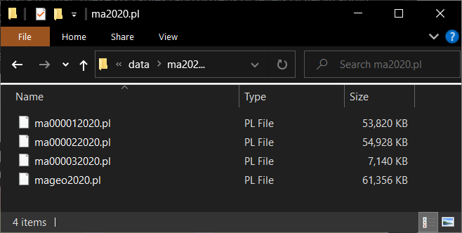
The legacy data format is available on the Census Bureau website. Each U.S. State has one zip file corresponding to it. Each zip file contains four distinct files. The legacy data contains six tables, five that contain population characteristics and one that contains housing characteristics (read more about that here). Those six tables are split across the four .pl files. Files 1 to 3 have the actual census data for each table. The geographic header, or the geo file, contains the identifiers such as the county/precinct IDs or FIPS codes. When you download a state's file, you should see something like this inside the zip file:
While the contents of these files differ, they will all have the same number of rows. The LOGRECNO column header in each file indicates the row number across each legacy data file.
Geographic Info
The Census Block is the smallest, or most specific, unit of spatial data by which Census information is organized. Yet, in the legacy data that is not the only data type we have access to. The Census has already done the hard work of structuring the data across every level of geography it typically uses.
That means that information might be duplicative. Meaning, that each of the six tables is broken down by spatial level. Those are:
- State
- County
- Census Tract
- Census Block Group
- Census Block
- Census Voting District
So, in order to access one of these specific spatial levels, you would need to create a subset of the larger combination dataset corresponding to the level of granularity you're seeking. This is coded in the SUMLEV column in the geographic header file.
Making the Legacy Data Usable
It's as simple as combining the columns across the four files to create the full P.L. 94-171 legacy data file. Here's what the workflow would look like:
- Read in the four legacy data files (we'll be working in R)
- Combine the four files into a single file, and subset the resulting dataset by a geography level.
- If need be, strip the data to only the desired variables for analysis.
- If need be, combine the resulting data with tigris shapefiles for mapping.
There are two distinct ways I've found that work well. I'll quickly walk through both of them.
Using the PL94171 Package
Created by Cory McCartan and Christopher Kenny, the PL94171 package for R streamlines access to P.L. 94-171 data. It's available on GitHub here.
Using the directory where I've stored the Massachusetts legacy data as an example, it's quite simple to import and use PL94171 to interface with the newly released data.
library(PL94171)

# `data/ma2020.pl` is a directory with the four P.L. 94-171 files for Massachusetts
pl_raw <- pl_read("data/ma2020.pl")
The above code block should be sufficient for creating a large list of four objects. Each object is an individual P.L. 94-171 file, but with PL94171, you're able to subset the entire list of four files according to one spatial/geographic level to access all the relevant information using the corresponding SUMLEV code.
> print(pl_geog_levels)
# A tibble: 85 x 2
   SUMLEV SUMLEV_description
   <chr>  <chr>
 1 040    State
 2 050    State-County
 3 060    State-County-County Subdivision
 4 067    State-County-County Subdivision-Subminor Civil Division
 5 140    State-County-Census Tract
 6 150    State-County-Census Tract-Block Group
 7 155    State-Place-County
 8 160    State-Place
 9 170    State-Consolidated City
10 172    State-Consolidated City-Place within Consolidated City
# ... with 75 more rows
So, if you wanted to filter the data by the Census Tract, you'd do the following:
> pl <- pl_subset(pl_raw, sumlev="140") # subset the data to census tracts
> print(dim(pl)) # print the dimensions of the resulting matrix
[1] 1620  397
That's it! You have usable data. If you wanted to further process the resulting dataset, you can use the pl_select_standard function with clean_names = TRUE in order to get both "standard set of basic population groups" and renamed columns to more comprehensible names.
pl_select_standard(pl, clean_names = TRUE)Using the Census Bureau's R Import Scripts
Normally, we'd be using the Census API or another library to access the relevant data in R. But while that information is not yet available in that format, the the Census Bureau released R import scripts that can be found here.
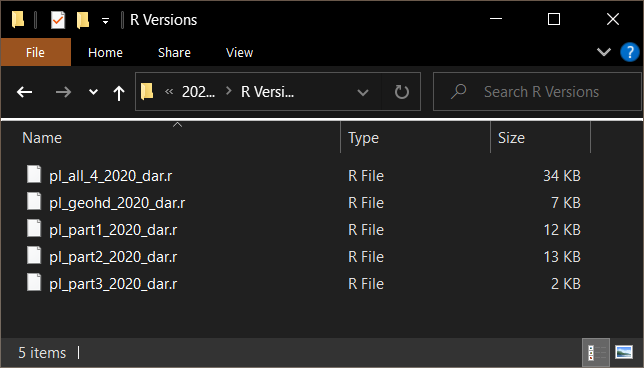
The above folder shows the five scripts available to us. Parts 1 to 3 allow us to create dataframes with just the individual files; geohd lets us access the geographic header information mentioned above, and the pl_all_4... file lets us access the entire dataset, and combine it into a single, very large dataframe.
I've found it to be quite simple to simply point your variables to where the four .pl files are located and simply run through the entire script. At the end, you should have an environment that looks like this:
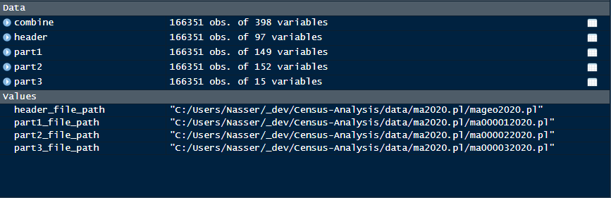
In combine we can see that there are 398 columns with 166351 rows. Just as the PL94171 package, you can subset this data to one spatial/geographic level to access all the relevant information using a corresponding SUMLEV code.
Note: unlike the PL94171 package, this will only subset the dataframe you choose. So if you subset combine, the other dataframes will not be effected.In R, you can just use dataframe indexing to create a subset:
# index to where SUMLEV == 140
ctract <- combine[combine$SUMLEV == 140,]

# Drop any columns where all values in the column are now null
str(ctract %>% select(where(not_all_na)))
That's it! Happy wrangling!